R Markdown files are a cross between markdown and R files since they can load and run chunks of code alongside markdown-formatted text.

• Benefits and downsides
• Parts
  • Header
  • Code chunks
  • Figures
  • Tables
  • References

Benefits and downsides

Benefits:

• Plots don’t need to be saved and loaded separately.
• Analysis is reproducible.
• Thanks to the markdown format, you can have nice equations with latex.
• Each chunk of code can be run separately to troubleshoot. This is more organized than using the console.

Downsides:

• you’ll have to load data every single time you knit the entire document. This can be really quite slow.
• Arranging the plots compactly still requires some work and controlling figure captions can be tricky. Sometimes you can’t determine formatting issues until you knit the whole thing.
• The comments in a code chunk are either all displayed, or all hidden; though sometimes you want some combination of both.

Parts

There is already a great R Markdown guide, I will just note a few points that I found helpful.

Header

When you setup the file, there are a couple of things you need to specify in the header. Most importantly, you need to specify the output format and the bibliography file (which should be in the same directory). For example, your header for a pdf document with tango color scheme highlights may proceed as follows:

---
title: "Stuff Goes here"
author: "Author"
date: "26/11/2019"
output:
  pdf_document: default
    highlight: tango
bibliography: report.bib
---

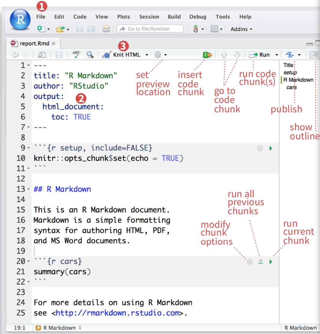
Code chunks

These are chunks of code that can be run separately or together. This image from the RStudio cheatsheet shows the general layout of the document, including the green arrows at the top of each chunk that can allow you to run it separately.

All of the formatting options must be specified into the chunk header. There is some description of the options in the Rmarkdown guide. Usually I have one chunk at the beginning of the document for loading all the libraries and setting directories, with the following simple setup which suppresses start up messages:

{r setup, include=FALSE}

This code chunk will not display in the main document. In general, it’s clunky to show the real code.

NOTE The chunk outputs such as figures and tables usually will display after the code, if you set both to display. However they can end up in unusual positions, appear out of order, and float around. To help with this, you can add the following to your startup chunk but it still may happen:

# this is meant to help the captions show up properly when you have a PDF output
opts_knit$set(eval.after = 'fig.cap') 
knitr::opts_chunk$set(fig.pos = 'H') #default figure position to be hold

It seems that the wierd positioning happens less with html output than pdf output.

Figures

To display figures, you can opt to show the figure but not the code by setting ‘echo=FALSE’. It works well to have one figure per chunk. In this way, you can add automatic figure references by adding a figure caption to the chunk header. Inside of the caption you may add the “label{fig:labelX}” to be able to refer back to this figure later. For example:

{r, fig.width=8, fig.height=1.5, echo=FALSE, fig.cap="\\label{fig:labelX} Caption goes here."}

When I knit the document with this chunk, a figure number and a figure caption will automatically appear next to the figure (below, by default). I can then make an inline reference to this figure as “Figure \ref{fig:labelX}” and the figure number will be automatically filled.

NOTE When you include more than one figure in a chunk, or if you mix a figure and a table, the document can glitch and the caption doesn’t show up sometimes. I’ve also seen this happen when you don’t leave enough space after a chunk.

Tables

To format a table to look good, you can use kable as a basic builtin option e.g. as follows. Note that kable includes an option to add a caption. When knit, a table number is automatically added in the caption.

kable(table(cars$speed/cars$dist),
      caption = "stuff")

However to make reference to this table you will need to include a figure caption in the chunk header. I haven’t figured out a way around this yet.

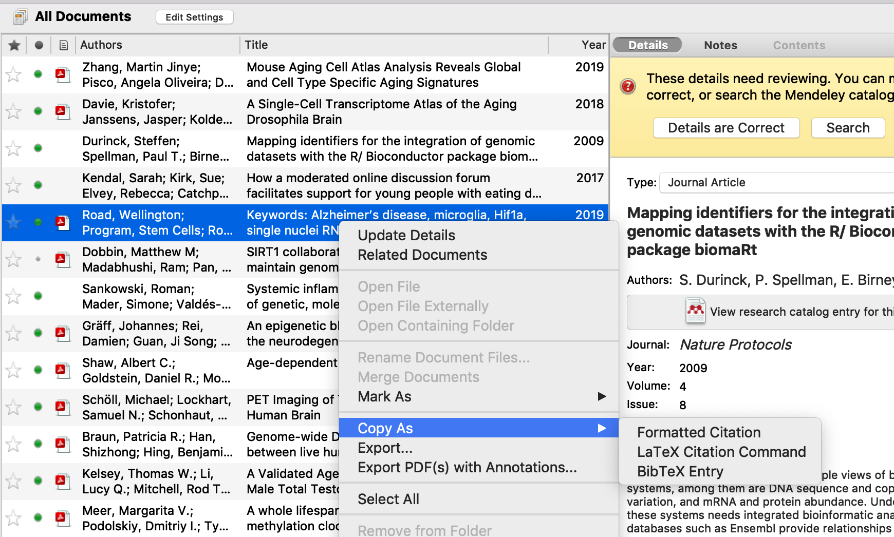
References

With the bibliography file you have specified in the header, you can include references inside the text in BibTex format. One easy way to export these references from Mendeley is to right click from the main menu and “copy as BibTex” as in the image below. Then you can paste into your bibliography file.